Analyzing R-loop data with RLSeq
29 September 2021
Abstract
This vignette covers basic usage of RLSeq for evaluating data quality and analyzing R-loop locations. RLSeq is part of RLSuite, an R-loop analysis toolchain. RLSuite also includes RLHub, RLBase (web interface), and RLPipes.
Package
RLSeq 0.9.0
1 Introduction

RLSeq is a package for analyzing R-loop mapping data sets, and it is a core component of the RLSuite toolchain. It serves two primary purposes: (1) to facilitate the evaluation of data quality, and (2) to enable R-loop data analysis in the context of genomic annotations and the public data sets in RLBase. The main analysis steps can be conveniently run using the RLSeq() function. Then, an HTML report can be generated using the report() function. Individual steps of this pipeline are also accessible through separate functions which provide custom analysis capabilities.
This vignette will showcase the primary functionality of RLSeq with data from a publicly-available R-loop data mapping study in Ewing sarcoma cell lines, GSE68845. We have selected two DNA-RNA Immunoprecipitation sequencing (DRIP-seq) samples for demonstration purposes: (1) SRX1025890, a positive R-loop mapping sample (“POS”; condition: S9.6 -RNaseH1), and (2) SRX1025892, a negative control (“NEG”; condition S9.6 +RNaseH1). We will begin by showing a quick-start analysis on SRX1025890, and then we will proceed to discuss, in detail, the specific steps of this analysis with both samples.
2 Quick-start
Here, we demonstrate a simple analysis workflow which utilizes a publicly-available data set stored in RLBase (a database R-loop-mapping experiments, also part of RLSuite). The commands below download these data, run RLSeq(), and generate the HTML report.
# Peaks and coverage can be found in RLBase
rlbase <- "https://rlbase-data.s3.amazonaws.com"
pks <- file.path(rlbase, "peaks", "SRX1025890_hg38.broadPeak")
cvg <- file.path(rlbase, "coverage", "SRX1025890_hg38.bw")

# Initialize data in the RLRanges object.
# Metadata is optional, but improves the interpretability of results
rlr <- RLRanges(
  peaks = pks,
  coverage = cvg,
  genome = "hg38",
  mode = "DRIP",
  label = "POS",
  sampleName = "TC32 DRIP-Seq"
)

# The RLSeq command performs all analyses
rlr <- RLSeq(rlr)

# Generate an html report
report(rlr, reportPath = "rlseq_report.html")
The report generated by this code is found here.
3 Preliminary
3.1 Installation
RLSeq should be installed alongside RLHub to facilitate access to the data required for annotation and analysis. When downloading RLSeq from bioconductor, RLHub is already included.
if (!requireNamespace("BiocManager", quietly = TRUE))
    install.packages("BiocManager")

BiocManager::install("RLSeq")
Both packages can also be installed from github.
library(remotes)
install_github("Bishop-Laboratory/RLHub")
install_github("Bishop-Laboratory/RLSeq")
3.2 Obtaining data
Obtaining data from raw files with RLPipes
RLSeq is compatible with R-loop data generated from a variety of pipelines and tools. However, it is strongly recommended that you use RLPipes, a snakemake-based CLI pipeline tool built specifically for upstream processing of R-loop datasets.
RLPipes can be installed using mamba or conda (slower).
# conda install -c conda-forge mamba
mamba create -n rlpipes -c bioconda -c conda-forge rlpipes
conda activate rlpipes
A typical config file CSV file should be written as such:
| experiment |
|---|
| SRX1025890 |
| SRX1025892 |
And then the pipeline can be run.
RLPipes build -m DRIP rseq_out/ tests/test_data/samples.csv
RLPipes run rseq_out/
The resulting directory will contain peaks/, coverage/, bam/, and other processed data sets which are directly compatible with RLSeq.
Note: If you choose to use a different pipeline, use macs2/macs3 for peak calling to ensure compatibility with RLBase.
4 End-to-end RLSeq
Here, we describe each step of the analysis pipeline which is run as part of the RLSeq() command.
4.1 Data sets
For this example, we will be using data from a 2018 Nature paper on R-loops in Ewing sarcoma (Gorthi et al. 2018). Two samples are used, one which has been IP’d for R-loops (S9.6 -RNaseH1; label: “POS”), and one which is the same, but with the addition of an RNaseH1 treatment (S9.6 +RNaseH1; label: “NEG”). RNaseH1 treatment degrades RNA:DNA hybrids (a core component of R-loops), so it serves as a useful negative control in these types of studies.
| experiment | condition |
|---|---|
| SRX1025890 | S9.6 - RNaseH1 |
| SRX1025892 | S9.6 + RNaseH1 |
The data was processed using RLPipes and uploaded to RLBase. Peaks are converted to GRanges objects using a helper function from regioneR.
rlbase <- "https://rlbase-data.s3.amazonaws.com"

# Get peaks and coverage
s96Pks <- regioneR::toGRanges(file.path(rlbase, "peaks", "SRX1025890_hg38.broadPeak"))
s96Cvg <- file.path(rlbase, "coverage", "SRX1025890_hg38.bw")
rnhPks <- regioneR::toGRanges(file.path(rlbase, "peaks", "SRX1025892_hg38.broadPeak"))
rnhCvg <- file.path(rlbase, "coverage", "SRX1025892_hg38.bw")
For demonstration purposes, only 10000 ranges from the positive (S9.6 -RNaseH1) sample are analyzed here.
# For expediency, peaks we filter and down-sampled to the top 10000 by padj (V9)
# This is not necessary as part of the typical workflow, however
s96Pks <- s96Pks[s96Pks$V9 > 2,]
s96Pks <- s96Pks[sample(names(s96Pks), 10000)]
Finally, RLRanges objects were constructed. These are the primary objects used in all RLSeq functions. RLRanges are an extension of GRanges which provide additional metadata and validation functions.
## Build RLRanges ##
# S9.6 -RNaseH1
rlr <- RLRanges(
  peaks = s96Pks,
  coverage = s96Cvg,
  genome = "hg38",
  mode = "DRIP",
  label = "POS",
  sampleName = "TC32 DRIP-Seq",
  quiet = TRUE
)

# S9.6 +RNaseH1
rlrRNH <- RLRanges(
  peaks = rnhPks,
  coverage = rnhCvg,
  genome = "hg38",
  mode = "DRIP",
  label = "NEG",
  sampleName = "TC32 DRIP-Seq (+RNaseH1)",
  quiet = TRUE
)
4.2 Sample quality
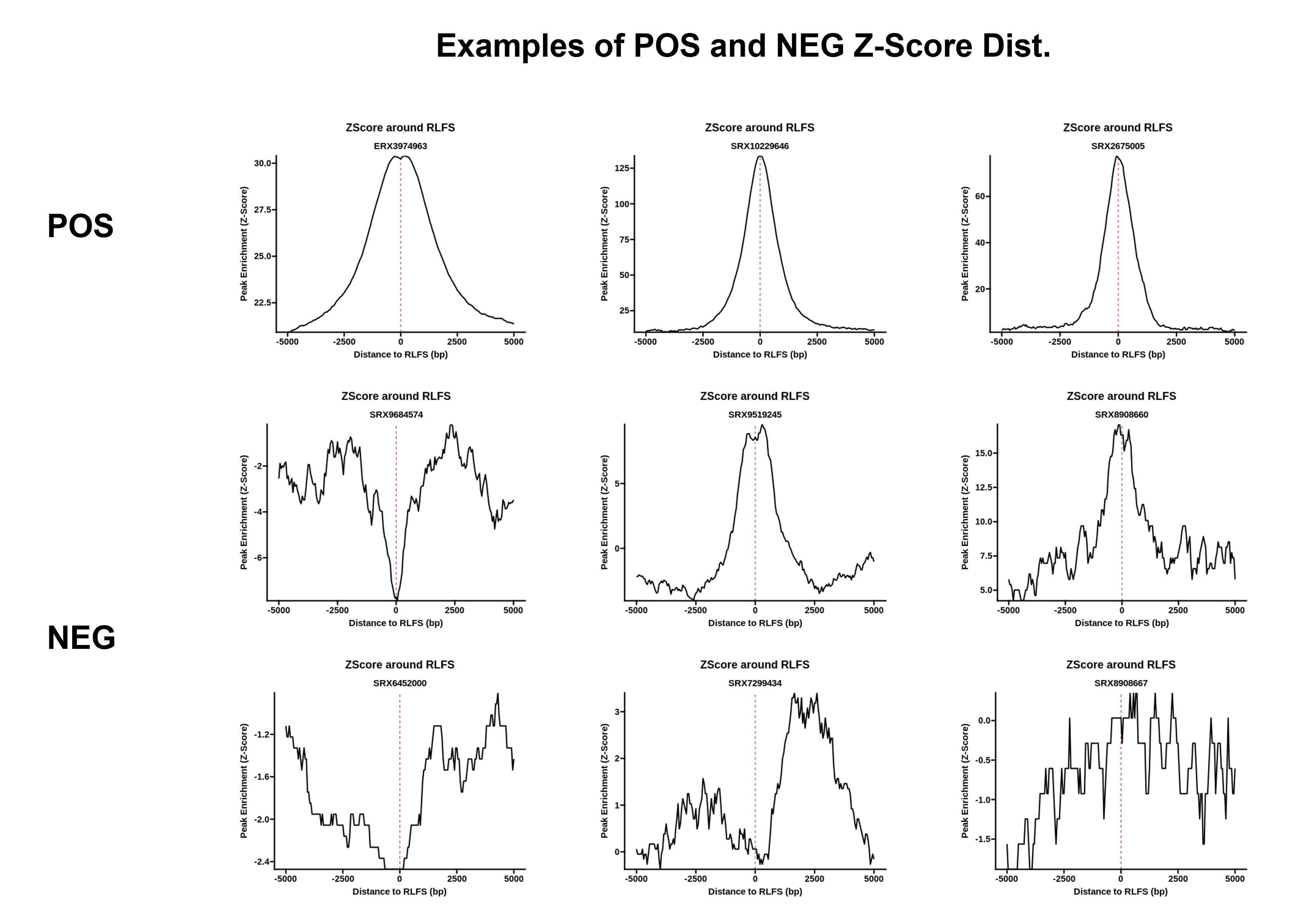
Sample quality is assessed by analyzing the association of peaks with R-loop-forming sequences (RLFS). RLFS are genomic sequences that favor the formation of R-loops (Jenjaroenpun et al. 2015). While R-loops can form outside RLFS, there is a noticeable relationship between R-loops and RLFS, which provides an unbiased test of whether a set of peaks actually represents successful R-loop mapping. This method is described in full within the RLSuite manuscript.
4.2.1 Permutation tests
RLSeq first implements a permutation test to evaluate the enrichment of peaks within RLFS and build a Z-score distribution around the TSS.
# Analyze RLFS for positive sample
rlr <- analyzeRLFS(rlr, quiet = TRUE)
rlrRNH <- analyzeRLFS(rlrRNH, quiet = TRUE)
The resulting objects now contain the permutation test results. These results can be easily visualized with the plotRLFSRes function.
plotRLFSRes(rlr)
Figure 1: Plot of permutation test results (S9.6 -RNaseH1)
As a comparison, we also view the negative control (S9.6 +RNaseH1) samples.
plotRLFSRes(rlrRNH)
Figure 2: Plot of permutation test results (S9.6 + RNaseH1)
From this example, we can see a fundamental challenge facing RLFS-based quality assessment: while the RNaseH1-treated sample is clearly a negative control, and the distribution does not resemble examples of positive samples found in RLBase (link), the p-value is still significant at p < 0.0099. This indicates that the p value from RLFS permutation testing is insufficient to distinguish successful and unsuccessful R-loop mapping. This observation motivated the development of a classifier model, which we made accessible within RLSeq.
4.2.2 Classifier predictions
The classifier is an ensemble model based on an online-learning scheme as detailed in the RLSuite manuscript. The latest version can be accessed via RLHub. To apply the model and predict sample quality, use the predictCondition() function.
# Predict
rlr <- predictCondition(rlr)
rlrRNH <- predictCondition(rlrRNH)
The results from testing our example samples:
# Access results
s96_pred <- rlresult(rlr, "predictRes")
rnh_pred <- rlresult(rlrRNH, "predictRes")

# Results
dplyr::tibble(
  condition = c("S9.6 -RNaseH1", "S9.6 + RNaseH1"),
  prediction = c(s96_pred$prediction, rnh_pred$prediction)
)
## # A tibble: 2 × 2
## condition prediction
## <chr> <chr>
## 1 S9.6 -RNaseH1 POS
## 2 S9.6 + RNaseH1 NEGThe resulting prediction from the model is either “POS” or “NEG”. POS means that the model predicts a sample is robustly mapping R-loops, whereas NEG samples are predicted to map R-loops poorly or not at all.
4.3 Feature enrichment
The feature enrichment test assesses the enrichment of genomic features within a supplied R-loop dataset. The function queries the RLHub annotation database to retrieve genomic features, and then it performs fisher’s exact test and the relative distance test to assess feature enrichment (Favorov et al. 2012).
# Perform test
rlr <- featureEnrich(
  object = rlr,
  quiet = TRUE
)
The results:
# View Top Results
annoResS96 <- rlresult(rlr, "featureEnrichment")
annoResS96 %>%
  relocate(contains("fisher"), .after = type) %>%
  arrange(desc(stat_fisher_rl))
## # A tibble: 50 × 13
## db type stat_fisher_rl stat_fisher_shuf pval_fisher_rl pval_fisher_shuf
## <chr> <chr> <dbl> <dbl> <dbl> <dbl>
## 1 Repeat… SINE Inf 1.01 4.51e-129 0.973
## 2 Transc… Intr… Inf 0.995 2.23e-308 0.801
## 3 Transc… Exon 20.9 1.04 2.23e-308 0.166
## 4 Transc… TTS 16.3 1.05 2.23e-308 0.180
## 5 Transc… TSS 15.6 1.06 2.23e-308 0.161
## 6 Encode… enhP 11.9 1.09 2.23e-308 0.0234
## 7 knownG… prot… 11.7 1.03 2.23e-308 0.152
## 8 snoRNA… CDBox 11.1 0.880 5.98e- 10 1
## 9 PolyA poly… 9.83 1.18 2.23e-308 0.0147
## 10 Transc… thre… 9.43 1.05 2.23e-308 0.460
## # … with 40 more rows, and 7 more variables: num_tested_peaks <int>,
## # num_total_peaks <int>, num_tested_anno_ranges <int>,
## # num_total_anno_ranges <int>, avg_reldist_rl <dbl>, avg_reldist_shuf <dbl>,
## # pval_reldist <dbl>From the results, we see that there is high enrichment within genic features, such as exons and introns.
RNaseH1 Comparison
As a comparison, we also performed the same test with the RNaseH1-treated sample.
# Perform test
rlrRNH <- featureEnrich(
  object = rlrRNH,
  quiet = TRUE
)
The results:
# View Top Results
annoResRNH <- rlresult(rlrRNH, "featureEnrichment")
annoResRNH %>%
  relocate(contains("fisher"), .after = type) %>%
  arrange(desc(stat_fisher_rl))
## # A tibble: 50 × 13
## db type stat_fisher_rl stat_fisher_shuf pval_fisher_rl pval_fisher_shuf
## <chr> <chr> <dbl> <dbl> <dbl> <dbl>
## 1 Repeat_Masker rRNA 12.7 0 6.09e- 5 1
## 2 Repeat_Masker tRNA 12.2 0 2.13e- 3 1
## 3 Repeat_Masker Retr… 11.9 0 8.47e- 18 1
## 4 Repeat_Masker Simp… 11.1 1.29 2.23e-308 0.0912
## 5 knownGene_RNAs rRNA… 10.9 0 1.50e- 2 1
## 6 Encode_CREs K4m3 8.05 0.709 5.22e- 48 0.347
## 7 skewr C_SK… 7.78 0.796 7.18e- 80 0.444
## 8 skewr G_SK… 7.36 1.14 3.16e- 76 0.510
## 9 Repeat_Masker Sate… 4.75 0.697 3.51e- 49 0.445
## 10 Repeat_Masker srpR… 3.82 0 2.31e- 1 1
## # … with 40 more rows, and 7 more variables: num_tested_peaks <int>,
## # num_total_peaks <int>, num_tested_anno_ranges <int>,
## # num_total_anno_ranges <int>, avg_reldist_rl <dbl>, avg_reldist_shuf <dbl>,
## # pval_reldist <dbl>Finally, we visualized the top results for the positive and negative conditions as a heat map.
inner_join(
  annoResRNH,
  annoResS96,
  by = c("db", "type"),
  suffix = c("__S9.6 +RNaseH1", "__S9.6 -RNaseH1")
) %>%
  select(db, type,  contains("stat_fisher_rl")) %>%
  tidyr::pivot_longer(cols = contains("__")) %>%
  mutate(
    group = gsub(name, pattern = ".+__(.+)$", replacement = "\\1"),
    value = ifelse(value == Inf, max(value[is.finite(value)]), value),
    value = log2(value)
  ) %>%
  filter(! is.na(value),
         is.finite(value)) %>%
  group_by(group) %>%
  filter(type %in% (slice_max(., order_by = value, n = 8) %>% pull(type))) %>%
  ungroup() %>%
  distinct(type, group, .keep_all = TRUE) %>%
  select(value, group, type) %>%
  tidyr::pivot_wider(id_cols = type, names_from = group,
                     values_from = value, values_fill = 0) %>%
  tibble::column_to_rownames(var = "type") %>%
  as.matrix() %>%
  ComplexHeatmap::pheatmap(
    color = colorRampPalette(RColorBrewer::brewer.pal("PuBuGn", n = 9))(100),
    main = "Top enriched features",
    name = "Fisher Log2 Ratio",
    angle_col = "45"
  )
4.3.1 Visualization of enrichment results
RLSeq provides a helper function, plotEnrichment, to facilitate the visualization of enrichment results.
pltlst <- plotEnrichment(rlr)This returns a list of plots named according to the corresponding annotation database. For example, Encode cis-regulatory elements (CREs):
pltlst$Encode_CREs
Using the splitby parameter
The splitby parameter allows for plotting with respect to prediction (predicted condition, ie, “POS” or “NEG”) or label (labeled condition). This can be useful when trying to determine whether a particular annotation is uniquely-enriched in samples which robustly map R-loops.
pltlst <- plotEnrichment(rlr, splitby = "prediction", pred_POS_only = FALSE)Encode cis-regulatory elements (CREs):
pltlst$Encode_CREs
Note: Caveat on data range
A limitation of this approach is that Fisher’s exact test sometimes returns Inf or -Inf for the statistic (odds ratio). While these results are useful in demonstrating robust enrichment or non-enrichment, they are difficult to plot in a meaningful way. As a compromise, plotEnrichment sets a limited data range of -10 through 15. These values were chosen because they encompass every finite value that can be returned from the implementation of Fisher’s test which RLSeq uses. In the above plots Inf results are shown on the y-axis at value 15 and, likewise, -Inf is shown at -10.
4.4 Correlation analysis
Correlation analysis finds inter-sample correlation coefficients of bin-level R-loop signal around gold-standard R-loop sites (sites profiled using ultra-long-read R-loop mapping – “SMRF-Seq”) (Chédin et al. 2021). This analysis helps to answer the question “how well does my data agree with previous results?”
rlr <- corrAnalyze(rlr)The results of this analysis are visualized using corrHeatmap.
corrHeatmap(rlr) These results demonstrate that our sample correlates well with similar DRIP-Seq data sets.
4.5 Gene Annotation
Gene annotations are automatically downloaded using AnnotationHub() and then intersected with RLRanges.
rlr <- geneAnnotation(rlr)Over-representation analysis
These results can then be used for over-representation analysis if desired. One caveat to this analysis is that the number of genes is a function of the number of peaks, and this can lead (at higher numbers) to noticeable bias in enrichment analysis.
len <- rlresult(rlr, "geneAnnoRes") %>%
  pull(gene_id) %>%
  unique() %>%
  length()
cat(len, " genes found in RLRanges")
## 5531 genes found in RLRangesTo address this, we filter RLRanges object to obtain the top 2000 ranges by p-adjusted value (qval in RLRanges objects.)
# Pull the peak names for the top 2000 peaks
topPks <- rlr %>%
  as.data.frame() %>%
  tibble::rownames_to_column(var = "peakName") %>%
  slice_max(qval, n = 2000) %>%
  pull(peakName)

# Filter the results to obtain the corresponding genes
rlgenes <- rlresult(rlr, "geneAnnoRes") %>%
  filter(peak_name %in% {{ topPks }}) %>%
  pull(gene_id) %>%
  unique()

# Get lenght of these genes
cat(length(rlgenes), " genes found in top 2000 RLRanges")
## 159 genes found in top 2000 RLRangesBefore we can perform pathway enrichment, we convert our gene IDs to gene symbols.
symbols <- AnnotationDbi::mapIds(
  org.Hs.eg.db::org.Hs.eg.db,
  keys = rlgenes,
  keytype = "ENTREZID",
  column = "SYMBOL"
)
With our final list of genes prepared, we proceed to perform over-representation analysis using the enrichr web service.
response <- httr::POST(
  url = 'https://maayanlab.cloud/Enrichr/addList',
  body = list(
    'list' = paste0(symbols, collapse = "\n"),
    'description' = paste0("RL-overlap Genes from ",
                           slot(rlr, "metadata")$sampleName)
  )
)
response <- jsonlite::fromJSON(httr::content(response, as = "text"))
permalink <- paste0(
  "https://maayanlab.cloud/Enrichr/enrich?dataset=", response$shortId[1]
)
The permalink to these results can be found here.
4.6 R-Loop Region Test
R-loop regions are consensus R-loop-forming sites discovered from analyzing all high-confidence R-loop mapping samples in RLBase. A description of this approach is found in the RLSuite manuscript. The rlRegionTest() analyzes the enrichment of the ranges in our RLRanges object with these consensus R-loop sites, which, like correlation analysis, also helps answer the question “how well does my data agree with previous results?”
rlr <- rlRegionTest(rlr)The test results can be easily visualized in the following manner.
plotRLRegionOverlap(
  object = rlr,

  # Arguments for VennDiagram::venn.diagram()
  fill = c("#9ad9ab", "#9aa0d9"),
  main.cex = 2,
  cat.pos = c(-40, 40),
  cat.dist=.05,
  margin = .05
)
5 Accessing RLBase data
For convenience, we also provide pre-analyzed RLRanges objects for every sample in RLBase. To access them, you need only provide the ID of the sample which you want to obtain data from. These IDs, along with other metadata, are listed in RLHub::rlbase_samples().
rlr <- RLRangesFromRLBase(acc = "SRX1025890")
rlr
## RLRanges object with 107029 ranges and 6 metadata columns:
## seqnames ranges strand | V4 V5 V6
## 1 chr1 10034-10345 * | /home/UTHSCSA/miller.. 40 .
## 2 chr1 180610-181657 * | /home/UTHSCSA/miller.. 53 .
## 3 chr1 182752-182950 * | /home/UTHSCSA/miller.. 38 .
## 4 chr1 184149-184628 * | /home/UTHSCSA/miller.. 28 .
## 5 chr1 629787-630103 * | /home/UTHSCSA/miller.. 42 .
## ... ... ... ... . ... ... ...
## 107025 chrY 11293162-11294964 * | /home/UTHSCSA/miller.. 38 .
## 107026 chrY 11295281-11296131 * | /home/UTHSCSA/miller.. 36 .
## 107027 chrY 11297625-11297944 * | /home/UTHSCSA/miller.. 23 .
## 107028 chrY 11301521-11301748 * | /home/UTHSCSA/miller.. 20 .
## 107029 chrY 26641735-26642007 * | /home/UTHSCSA/miller.. 15 .
## V7 V8 qval
## 1 4.17431 6.16893 4.04326
## 2 4.63235 7.59510 5.31977
## 3 4.21966 5.95157 3.81400
## 4 3.57860 4.84694 2.87393
## 5 2.59231 6.38817 4.27687
## ... ... ... ...
## 107025 2.33249 5.86578 3.81115
## 107026 2.18689 5.72732 3.67967
## 107027 2.45115 4.20891 2.32963
## 107028 2.98060 3.91975 2.09600
## 107029 2.80910 3.30759 1.56104
##
## SRX1025890:
## Mode: DRIP
## Genome: hg38
## Label:
##
## RLSeq Results Available:
## featureEnrichment, correlationMat, rlfsRes, geneAnnoRes, predictRes, rlRegionRes
##
## prediction:6 Session
Session info
sessionInfo()## R version 4.1.1 (2021-08-10)
## Platform: x86_64-pc-linux-gnu (64-bit)
## Running under: Ubuntu 20.04.3 LTS
##
## Matrix products: default
## BLAS: /usr/lib/x86_64-linux-gnu/blas/libblas.so.3.9.0
## LAPACK: /usr/lib/x86_64-linux-gnu/lapack/liblapack.so.3.9.0
##
## locale:
## [1] LC_CTYPE=en_US.UTF-8 LC_NUMERIC=C
## [3] LC_TIME=en_US.UTF-8 LC_COLLATE=en_US.UTF-8
## [5] LC_MONETARY=en_US.UTF-8 LC_MESSAGES=en_US.UTF-8
## [7] LC_PAPER=en_US.UTF-8 LC_NAME=C
## [9] LC_ADDRESS=C LC_TELEPHONE=C
## [11] LC_MEASUREMENT=en_US.UTF-8 LC_IDENTIFICATION=C
##
## attached base packages:
## [1] stats graphics grDevices utils datasets methods base
##
## other attached packages:
## [1] RLHub_0.9.0 dplyr_1.0.7 RLSeq_0.9.0 BiocStyle_2.21.3
##
## loaded via a namespace (and not attached):
## [1] utf8_1.2.2 tidyselect_1.1.1
## [3] RSQLite_2.2.8 AnnotationDbi_1.55.1
## [5] grid_4.1.1 BiocParallel_1.27.10
## [7] pROC_1.18.0 devtools_2.4.2
## [9] aws.signature_0.6.0 munsell_0.5.0
## [11] codetools_0.2-18 future_1.22.1
## [13] withr_2.4.2 colorspace_2.0-2
## [15] Biobase_2.53.0 filelock_1.0.2
## [17] highr_0.9 knitr_1.34
## [19] rstudioapi_0.13 stats4_4.1.1
## [21] listenv_0.8.0 MatrixGenerics_1.5.4
## [23] labeling_0.4.2 GenomeInfoDbData_1.2.7
## [25] bit64_4.0.5 farver_2.1.0
## [27] rprojroot_2.0.2 parallelly_1.28.1
## [29] vctrs_0.3.8 generics_0.1.0
## [31] lambda.r_1.2.4 ipred_0.9-12
## [33] xfun_0.26 BiocFileCache_2.1.1
## [35] regioneR_1.25.1 R6_2.5.1
## [37] doParallel_1.0.16 GenomeInfoDb_1.29.8
## [39] clue_0.3-59 gridGraphics_0.5-1
## [41] bitops_1.0-7 cachem_1.0.6
## [43] DelayedArray_0.19.4 assertthat_0.2.1
## [45] promises_1.2.0.1 BiocIO_1.3.0
## [47] scales_1.1.1 nnet_7.3-16
## [49] gtable_0.3.0 globals_0.14.0
## [51] processx_3.5.2 timeDate_3043.102
## [53] rlang_0.4.11 GlobalOptions_0.1.2
## [55] splines_4.1.1 rtracklayer_1.53.1
## [57] ModelMetrics_1.2.2.2 BiocManager_1.30.16
## [59] yaml_2.2.1 reshape2_1.4.4
## [61] httpuv_1.6.3 caret_6.0-88
## [63] tools_4.1.1 lava_1.6.10
## [65] usethis_2.0.1 bookdown_0.24
## [67] ggplotify_0.1.0 ggplot2_3.3.5
## [69] ellipsis_0.3.2 jquerylib_0.1.4
## [71] RColorBrewer_1.1-2 BiocGenerics_0.39.2
## [73] sessioninfo_1.1.1 Rcpp_1.0.7
## [75] plyr_1.8.6 base64enc_0.1-3
## [77] zlibbioc_1.39.0 purrr_0.3.4
## [79] RCurl_1.98-1.5 ps_1.6.0
## [81] prettyunits_1.1.1 rpart_4.1-15
## [83] pbapply_1.5-0 GetoptLong_1.0.5
## [85] S4Vectors_0.31.3 SummarizedExperiment_1.23.4
## [87] cluster_2.1.2 fs_1.5.0
## [89] magrittr_2.0.1 data.table_1.14.0
## [91] futile.options_1.0.1 magick_2.7.3
## [93] caretEnsemble_2.0.1 circlize_0.4.13
## [95] matrixStats_0.61.0 pkgload_1.2.2
## [97] mime_0.11 evaluate_0.14
## [99] xtable_1.8-4 XML_3.99-0.8
## [101] VennDiagram_1.6.20 IRanges_2.27.2
## [103] gridExtra_2.3 shape_1.4.6
## [105] testthat_3.0.4 compiler_4.1.1
## [107] tibble_3.1.4 crayon_1.4.1
## [109] htmltools_0.5.2 later_1.3.0
## [111] ggprism_1.0.3 tidyr_1.1.3
## [113] lubridate_1.7.10 aws.s3_0.3.21
## [115] DBI_1.1.1 formatR_1.11
## [117] ExperimentHub_2.1.4 dbplyr_2.1.1
## [119] ComplexHeatmap_2.9.4 MASS_7.3-54
## [121] rappdirs_0.3.3 Matrix_1.3-4
## [123] cli_3.0.1 parallel_4.1.1
## [125] gower_0.2.2 GenomicRanges_1.45.0
## [127] pkgconfig_2.0.3 GenomicAlignments_1.29.0
## [129] recipes_0.1.16 xml2_1.3.2
## [131] foreach_1.5.1 bslib_0.3.0
## [133] XVector_0.33.0 prodlim_2019.11.13
## [135] yulab.utils_0.0.2 stringr_1.4.0
## [137] callr_3.7.0 digest_0.6.28
## [139] Biostrings_2.61.2 rmarkdown_2.11
## [141] restfulr_0.0.13 curl_4.3.2
## [143] shiny_1.7.0 Rsamtools_2.9.1
## [145] rjson_0.2.20 lifecycle_1.0.1
## [147] nlme_3.1-153 jsonlite_1.7.2
## [149] futile.logger_1.4.3 desc_1.3.0
## [151] BSgenome_1.61.0 fansi_0.5.0
## [153] pillar_1.6.2 lattice_0.20-44
## [155] KEGGREST_1.33.0 fastmap_1.1.0
## [157] httr_1.4.2 pkgbuild_1.2.0
## [159] survival_3.2-13 interactiveDisplayBase_1.31.2
## [161] glue_1.4.2 remotes_2.4.0
## [163] png_0.1-7 iterators_1.0.13
## [165] BiocVersion_3.14.0 bit_4.0.4
## [167] class_7.3-19 stringi_1.7.4
## [169] sass_0.4.0 blob_1.2.2
## [171] AnnotationHub_3.1.5 memoise_2.0.0
## [173] future.apply_1.8.1